Recent Posts (page 2 / 8)

Distribute MATLAB Computations To Python Running on a Cluster with Dask

Part 12 of the Python Is The Ultimate MATLAB Toolbox series.

Introduction

My previous post, Accelerate MATLAB with Python and Numba, showed how compute-bound MATLAB applications can be made to run faster if slow MATLAB operations are rewritten in Python. If the resulting speed improvement isn’t enough, different hardware architectures like GPUs or a cluster of computers may be your only recourse for even higher performance. MATLAB has both of these nailed—if you have the Parallel Computing Toolbox and the necessary hardware.

If you don’t have access to this toolbox but you do have ssh access to a collection of computers and you’re willing to include Python in your MATLAB workflow, the dask module can help your MATLAB application tap into those computers' collective CPU power.

• Prerequisites
• Start the dask cluster
• Example 1: sum of prime factors
• Example 2: gigapixel Mandelbrot image
• Example 3: finite element frequency domain response

Prerequisites

Although dask can run on the cores of a single computer, in this article I’ll cover dask’s ability to send computations to, and collect results from a group of remote computers. This raises a few complications: to use dask with a remote computer you’ll need to have an account on it and be able to send commands to it without entering a password. Further, the remote computer should have enough network, file storage, memory, and CPU resources necessary to run your computations. In particular, do you need to share the remote computer with others?

Many organizations with sizeable engineering or research departments operate compute clusters explicitly to enable large scale parallel computations. Access and resource sharing are done with job schedulers such as LSF, PBS, or Slurm. Dask has interfaces to these but here I’ll work with the most simple setups of all, a group of individual computers on which I have accounts and can access through ssh. Here’s the full list of prerequisites:

• compatible (preferrably identical) Python installations including dask, distributed, and paramiko modules
• the same path to the Python executable
• the same account name for the user setting up and using the cluster
• uniform bi-directional, key-based ssh access across all computers for the user account
• same ssh port
• firewall rules open to allow ssh and the dask scheduler and metrics ports (8786 and 8787 by default)

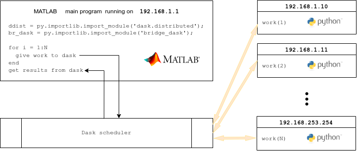
Start the dask cluster

Each computer that is to participate in your computations needs to have a dask worker process running on it. Additionally, one of the computers must run the dask scheduler process. These processes can be started with ssh, Kubernetes, Helm, or any of the job schedulers (LSF, etc) mentioned above. Any method other than ssh, however, will likely require help from a cluster administrator or tech support expert.

I’ll avoid complications and only describe the ssh method.

Note: the method described below of starting a dask cluster with dask-ssh --hostfile is insecure because anyone with access to the computers and knowledge of the dask port can submit jobs as though they were you. The secure way to set up a dask cluster is with a dask gateway.

Start by creating a text file with each host’s IP address (or hostname, if name resolution works) on a single line. The file might look like this

# file: my_hosts.txt
127.0.0.1
192.168.1.39
192.168.1.40
192.168.1.41
192.168.1.65

Hostnames may be repeated. I typically run with a file that defines only localhost entries such as

# file: my_hosts.txt
127.0.0.1
127.0.0.1
127.0.0.1

while I’m developing a parallel program. I only submit to remote computers after I’m convinced the code works locally.

Next, pass the file of host names to the dask-ssh command to start the worker on each node, and also a scheduler:

dask-ssh --hostfile my_hosts.txt

You’ll see a stream of messages resembling

---------------------------------------------------------------
                 Dask.distributed v2022.7.0

Worker nodes: 3
  0: 127.0.0.1
  1: 127.0.0.1
  2: 127.0.0.1

scheduler node: 127.0.0.1:8786
---------------------------------------------------------------


/usr/local/anaconda3/2021.05/lib/python3.8/site-packages/paramiko/transport.py:219: CryptographyDeprecationWarning: Blowfish has been deprecated
  "class": algorithms.Blowfish,
[ scheduler 127.0.0.1:8786 ] : /usr/local/anaconda3/2021.05/bin/python -m distributed.cli.dask_scheduler --port 8786
                                      :
                                (lines deleted)
                                      :
INFO - Register worker <WorkerState 'tcp://127.0.0.1:37661', status: init, memory: 0, processing: 0>
[ scheduler 127.0.0.1:8786 ] : 2022-11-07 20:58:36,128 - distributed.scheduler - INFO - Starting worker compute stream, tcp://127.0.0.1:37661
[ scheduler 127.0.0.1:8786 ] : 2022-11-07 20:58:36,129 - distributed.core - INFO - Starting established connection

Note line of output with scheduler node: 127.0.0.1:8786. This is the host and port where the scheduler listens for instructions. We’ll need this value to create a dask client (described below).

The dask-ssh command will tie up your terminal until the cluster is shut down. That can be done by entering ctrl-c in the terminal.

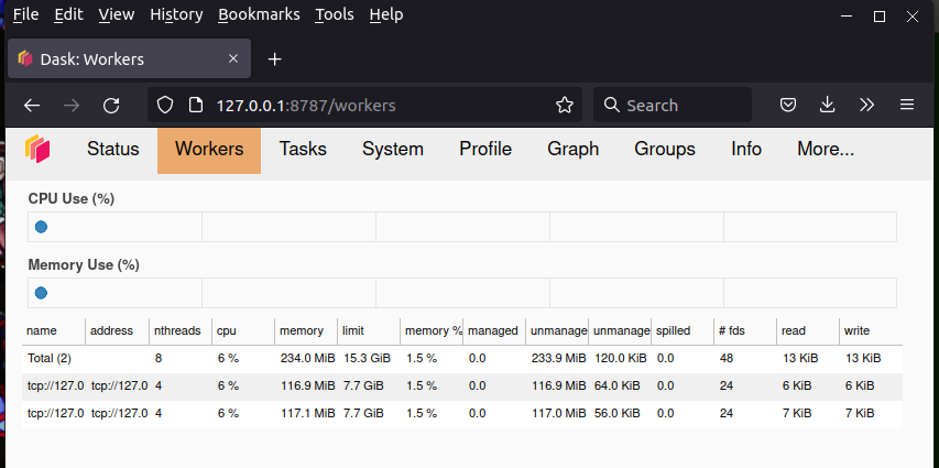
The dask scheduler runs a web server that shows lots of useful information about the state of your cluster. View it by entering your scheduler node’s hostname or IP address followed by :8787 as a URL in your browser. In my case that’s http://127.0.0.1:8787 or http://localhost:8787. The view under the Workers tab looks like this:

Track your compute nodes on this web while dask is cranking away at one of the following examples, all of which come from the High Performance Computing chapter of my book.

Example 1: sum of prime factors

I’ll start with a simple example to demonstrate the mechanics of using dask. The Python and MATLAB programs below compute the sum of unique prime factors of all numbers in a given range. The hard part, computing the prime factors themselves, is done with SymPy’s primefactors() function, comparable to MATLAB’s factor()¹.

Here are sequential implementations:

Python:

 1
 2
 3
 4
 5
 6
 7
 8
 9
10
11
12
13
14
15
16
17
18
19

#!/usr/bin/env python3
# file: prime_seq.py
from sympy import primefactors
import time
def my_fn(a, b, incr):
    Ts = time.time()
    s = 0
    for x in range(a,b,incr):
        s += sum(primefactors(x))
    return s, time.time() - Ts
def main():
    A = 2
    B = 10_000_000
    incr = 1
    S, dT = my_fn(A, B, incr)
    print(f'A={A} B={B} {dT:.4f} sec')
    print(f'S={S}')
if __name__ == "__main__": main()

MATLAB:

 1
 2
 3
 4
 5
 6
 7
 8
 9
10
11
12
13
14
15

% file: prime_seq.m
A = 2;
B = 10000000;
incr = 1;
[S, dT] = my_fn(A, B, incr);
fprintf('A=%d B=%d, %.3f sec\n', A, B, dT);
fprintf('S=%ld\n', S);
function [S, dT]=my_fn(A, B, incr)
    tic;
    S = 0;
    for i = A:incr:B-1
        S = S + sum(unique(factor(i)));
    end
    dT = toc;
end

Performance looks like this on my laptop:

Calls to the compute intensive function my_fn() are independent and can be called in any order, or even simultaneously. We’ll do exactly that with dask, using three cores of the local machine. To spread the load evenly we merely need to offset the first number in the sequence by the job number, 0 to N-1 for N jobs, then stride through the sequence in steps of N. For example if we compute prime factors for numbers between 2 and 20 and want to spread the work evenly over three jobs, the assignments will be

In : list(range(2,21))            # original set
Out: [2, 3, 4, 5, 6, 7, 8, 9, 10, 11, 12, 13, 14, 15, 16, 17, 18, 19, 20]

In : list(range(2+0,21,3))        # for processor 1 (does job 0)
Out: [2, 5, 8, 11, 14, 17, 20]

In : list(range(2+1,21,3))        # for processor 2 (does job 1)
Out: [3, 6, 9, 12, 15, 18]

In : list(range(2+2,21,3))        # for processor 3 (does job 2)
Out: [4, 7, 10, 13, 16, 19]

or, equivalently in MATLAB,

>> 2+0:3:20                       % for processor 1 (does job 0)
     2     5     8    11    14    17    20

>> 2+1:3:20                       % for processor 2 (does job 1)
     3     6     9    12    15    18

>> 2+2:3:20                       % for processor 3 (does job 2)
     4     7    10    13    16    19

The dask-enabled version of the prime factor summation program on the local computer, splitting up the work to three tasks that are to run simultaneously, looks like this:

 1
 2
 3
 4
 5
 6
 7
 8
 9
10
11
12
13
14
15
16
17
18
19
20
21
22
23
24
25
26
27
28
29
30
31
32
33
34
35
36

#!/usr/bin/env python3
# file: prime_dask.py
from sympy import primefactors
import time
import dask
from dask.distributed import Client

def my_fn(a, b, incr):
    Ts = time.time()
    s = 0
    for x in range(a,b,incr):
        s += sum(primefactors(x))
    return s, time.time() - Ts

def main():
    client = Client('127.0.0.1:8786')
    tasks  = []
    main_T_start = time.time()
    n_jobs = 3
    A = 2
    B = 10_00 # 0_000
    incr = n_jobs
    for i in range(n_jobs):
        job = dask.delayed(my_fn)(A+i, B, incr)
        tasks.append(job)
    results = dask.compute(*tasks)
    client.close()
    total_sum = 0
    for i in range(len(results)):
        partial_sum, T_el = results[i]
        print(f'job {i}:  sum= {partial_sum}  T= {T_el:.3f}')
        total_sum += partial_sum
    print(f'total sum={total_sum}')
    elapsed = time.time() - main_T_start
    print(f'main took {elapsed:.3f} sec')
if __name__ == "__main__": main()

Lines 5, 6 import the dask module and the Client class

Line 16 Creates a Client object that connects to the dask scheduler on the cluster we set up earlier.

Line 17 Initializes an empty list that will later store “tasks”, basically a unit of work made of a function to call and its input arguments.

Line 19 defines the number of chucks we’ll subdivide the work into. This number should match or exceed the number of dask workers, in other words, the number of remote computers we can run on.

Lines 23-25 populates the task list. Each entry, “job”, is an invocation of my_fn() with input arguments that stride between A and B so as to span a unique collection of numbers.

Line 26 tells the scheduler to send the tasks to the workers to begin performing the computations. The return value from each task comes back as the list results.

Line 27 is reached when the last worker has finished.

Lines 28-32 fetches the solution for each task and adds it to the global sum variable.

With the scheduler and workers running in the background, we can now run the dask-enabled prime factor summation program prime_dask.py. It runs faster than the sequential version, but not by much:

3 worker processes, 3 dask jobs:
job 0: sum= 2418248946959 T= 327.969
job 1: sum= 659400211060 T= 206.228
job 2: sum= 2417852197037 T= 327.709
total sum=5495501355056
main took 328.852 sec

Performance disappoints for two reasons. First, the workload is clearly imbalanced since one job took around 200 seconds, while the other two took more than 320. Evidently, terms of the sequence 3, 6, 9 … can be factored much more rapidly than terms in 2, 5, 8 … and 4, 7, 10 …—who knew? The second reason is less obvious. It is that the sum of individual core times, 328.0 + 206.2 + 327.7 = 861.9 seconds, is 66% higher than the single-core time of 519.5 seconds. Clearly there’s a non-trivial overhead to using dask.

Parallel prime factor summation in MATLAB

Now that we can run our Python program in parallel with dask, we can do the same thing in MATLAB—with a couple of restrictions:

1. Tasks submitted to dask must be Python functions. Therefore our MATLAB main program will need to send the Python version of the compute function, my_fn() in this example, to the remote workers.
2. MATLAB cannot call the dask.delayed() and dask.compute() functions directly. In particular, the asterisk in the call to dask.compute() (see line 26 in the listing above) is not legal MATLAB syntax. We’ll need a small Python bridge module to overcome these limitations.

The first restriction isn’t a big deal for this example; we merely need to import my_fn() from prime_seq.py or prime_dask.py. For a more substantial MATLAB application, though, this could mean translating a lot of MATLAB code to Python.

Aside: bridge_dask.py

The second restriction is easily resolved with just a few lines of Python:

1
2
3
4
5
6

# file: bridge_dask.py
import dask
def delayed(Fn, *args):
    return dask.delayed(Fn)(*args);
def compute(delayed_tasks):
    return dask.compute(*delayed_tasks)

This simple module provides wrappers to dask.delayed() and dask.compute() in a form suitable for MATLAB.

Parallel prime factor summation in MATLAB, continued

We now have the pieces in place to have MATLAB send the prime factor computation and summation work to a cluster of workers. The solution looks like this:

 1
 2
 3
 4
 5
 6
 7
 8
 9
10
11
12
13
14
15
16
17
18
19
20
21
22
23
24
25
26
27
28
29
30
31
32
33
34
35

% file: prime_dask.m
ddist = py.importlib.import_module('dask.distributed');
prime_seq = py.importlib.import_module('prime_seq');
br_dask = py.importlib.import_module('bridge_dask');

A = int64(2);
B = int64(10000000);
n_jobs = int64(3);

tic;
client = ddist.Client('127.0.0.1:8786');
client.upload_file('prime_seq.py');

% submit the jobs to the cluster
tasks = py.list({});
incr = n_jobs;
for i = 0:n_jobs-1
    task = br_dask.delayed(prime_seq.my_fn, A+i, B, incr);
    tasks.append(task);
end
results = br_dask.compute(tasks);  % start the computations, insert each
client.close()                     % worker's solution to the list 'results'
% gets here after all remote workers have finished

% post-processing:  aggregate the partial solutions
S = 0;
mat_results = py2mat(results);
for i = 1:length(mat_results)
    partial_sum = mat_results{i}{1};
    S = S + partial_sum;
    fprintf('Job %d took %.3f sec\n', i-1, mat_results{i}{2});
end
dT = toc;
fprintf('A=%d B=%d, %.3f sec\n', A, B, dT);
fprintf('S=%ld\n', S);

Line 12 has an important we didn’t need in the pure Python solution: it uploads our Python module file to the workers. Keep in mind that the workers do not share memory or file resources with the main program and therefore need to be given all items, whether input data or our code files, to function properly. (Incidentally, the upload_file() function can only be used to send source files to the workers. A different function, demonstrated in Example 3, is needed for other files.)

Our bridge module functions are called at lines 18 and 21. Line 26 calls the py2mat.m function to convert the Python solution list into a MATLAB cell array.

MATLAB’s parallel performance matches Python’s—mediocre, not great:

>> prime_dask
Job 0 took 345.014 sec
Job 1 took 219.340 sec
Job 2 took 344.900 sec
A=2 B=10000000, 345.164 sec
S=5495501355056

Nonetheless we’ve established the mechanics of sending computations from a MATLAB main program to a collection of Python workers and getting the results back as native MATLAB variables.

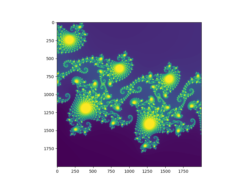
Example 2: gigapixel Mandelbrot image

My second example does a bit more interesting work in a bit more interesting fashion: I’ll scale up the Mandelbrot set example from 5,000 x 5,000 pixels to 35,000 x 35,000—more than 1.2 billion pixels. This is 49x larger than the 5k x 5k image so we can expect it to take 49x longer—several minutes instead of several seconds. This time I’ll farm the work out to actual remote computers, a collection of 18 virtual machine instances from DigitalOcean². Foolishly, perhaps, I start the dask cluster when I need it using the insecure dask-ssh --hostname method.

I had to restructure the solution to work on the memory limited workers. Instead of simply subdividing my 35,000 x 35,000 frame across the 18 workers, I had to go an extra step and first break the frame into smaller sub-frames, spread each sub-frame across the 18 workers, harvest the results from the sub-frame, then send the next sub-frame out. The code below uses the term group to refer to a sub-frame:

MATLAB:

 1
 2
 3
 4
 5
 6
 7
 8
 9
10
11
12
13
14
15
16
17
18
19
20
21
22
23
24
25
26
27
28
29
30
31
32
33
34
35
36
37
38
39
40
41
42
43
44
45
46

% file: MB_dask.m
ddist = py.importlib.import_module('dask.distributed');
np    = py.importlib.import_module('numpy');
MB_py = py.importlib.import_module('MB_numba_dask');
br_dask = py.importlib.import_module('bridge_dask');

N = int64( 35000 );
imax = int64(255);
Tc = tic;
nR = N; nC = N;
Re_limits = np.array({-0.7440, -0.7433});
Im_limits = np.array({ 0.1315,  0.1322});
n_groups = 16;
n_jobs_per_group = 18;
n_jobs = n_jobs_per_group*n_groups;
client = ddist.Client('127.0.0.1:8786'); % replace with scheduler IP
client.upload_file('MB_numba_dask.py');
results = py.list({});
for c = 1:n_groups
  tasks  = py.list({});
  Tcs = tic;
  for i = 1:n_jobs_per_group
    job_id = int64((c-1)*n_jobs_per_group+i-1);
    task = br_dask.delayed(MB_py.MB, nC, Re_limits, ...
        nR, Im_limits, imax, job_id, n_jobs);
    tasks.append(task);
  end
  results.extend( br_dask.compute(tasks) );
  Tce = toc(Tcs);
  fprintf('group %2d took %.3f sec\n', c-1, Tce)
end
client.close();

% reassemble the image
img = zeros(N,N, 'uint8');
Tps = tic;
for i = 1:length(results)
  my_rows  = py2mat(results{i}{1}) + 1; % 0-indexing to 1
  img_rows = py2mat(results{i}{2});
  img(my_rows,:) = img_rows;
end
Tpe = toc(Tps);
fprintf('py2mat conversion took %.3f\n', Tpe);
Te = toc(Tc);
fprintf('%.3f  %5d\n', Te, N);
imshow(img)

Line 4 imports the Numba-powered Mandelbrot functions from the file MB_numba_dask.py. The MB() function in this file differs a bit from the one in the Python+Numba article. This MB() figures out which rows of the sub-frame to stride over then returns the indices of these rows to the caller so that the caller can reassemble the overall frame more easily.

Line 16 shows the IP address of the localhost. In reality, I use the IP address of the DigitalOcean instance running my dask scheduler. I won’t advertise this address to keep my instances from unnecessary attention.

Line 17 uploads the MB_numba_dask.py module file to the workers.

The loop starting at line 19 iterates over the 16 sub-frames. I further divide each sub-frame across 18 workers so a worker at any one time is only doing math on 35000/(18*16), or roughly 122 rows at a time (each of which has 35000 columns).

Line 28 collects the results for the sub-frame from the 18 workers, then the loop continues to the next sub-frame.

Line 38 and 39 convert the Python numeric solution into native MATLAB variables. These are expensive steps because more than a gigabyte of data has to be copied.

Line 46 displays the resulting image, which doesn’t seem noteworthy. It is, though. MATLAB on an 8 GB laptop can comfortably render the gigapixal image whereas matplotlib’s equivalent command, plt.imshow() crashes.

Here are performance numbers for a typical run:

>> MB_numba_dask
group 0 took 5.658 sec
group 1 took 6.278 sec
group 2 took 4.812 sec
group 3 took 5.495 sec
group 4 took 4.746 sec
group 5 took 5.028 sec
group 6 took 4.982 sec
group 7 took 5.098 sec
group 8 took 4.911 sec
group 9 took 5.036 sec
group 10 took 4.923 sec
group 11 took 4.790 sec
group 12 took 4.946 sec
group 13 took 4.530 sec
group 14 took 4.528 sec
group 15 took 5.192 sec
py2mat conversion took 30.253
111.463 35000

In other words, just under 2 minutes to get results when running on 18 computers compared to an estimated 46 minutes for a pure MATLAB solution running on a single computer (56.77 seconds for 5k x 5k * 49 larger problem / 60 sec/min). True, much of the performance comes just from Numba. However the DigitalOcean virtual machines have just one core each and these run much slower than the cores of my laptop. I can’t run MATLAB on the virtual machines so it is difficult to separate know what my parallel efficiency is.

Example 3: finite element frequency domain response

Few real-world problems are as clean to set up and solve as the previous two examples. Realistic tasks typically involve substantial amounts of input data and then create volumes of new data. Figuring out how to split, transfer, then reassemble data efficiently can be as difficult as designing algorithms that can run in parallel. Often, as in this next example, you have to decide whether to transfer data from the main program to the remote workers or have all the workers perform duplicate work to generate the same data. The problem is compounded when using MATLAB with dask because you’ll also need to decide how much of your MATLAB code you’re willing to reimplement in Python for execution on the remote computers.

This example comes from the field of structural dynamics. It solves a system of equations involving stiffness ($K$), damping ($C$), and mass matrices ($M$) from a finite element discretization of a structure at many frequencies $\omega_k$, where $k$ = 1 .. $N$:

$$ K x_k + i \omega_k C x_k - \omega_k^2 M x_k = P(\omega_k) b $$

$N$ is typically in the hundreds but can exceed a thousand if the frequency content of the load spectrum, $P(\omega_k)$, spans a wide range. The vector $b$ stores the static load at each degree of freedom.

If the finite element model is large, each individual solution will take minutes (or worse!). Scale that by $N$ and you’ll be waiting a while for answers, possibly a very long while. The problem is easily divided among processors, however, since each frequency’s solution is independent of the other frequencies.

The first design decision to make is should we 1) compute $K$, $C$, and $M$ in the main program, written in MATLAB, then copy the matrices to the remote computers for solution in Python, or 2) send the model description to the remote computers and have them independently regenerate $K$, $C$, and $M$, then solve them at a subset of frequencies?

The second method involves much less network traffic but it also means translating the MATLAB finite element generation and assembly routines to Python. The first method puts a big load on the network to transfer the large matrices to many remote computers but it also means there’s little extra code to write; Python already has fast linear equation solvers for dense and sparse matrices. I’ll choose the lazy “write less code” option, method 1, in this case.

Chapter 14 of my book describes the full finite element solver using sparse matrices implemented in both MATLAB and Python and includes representative models of a notional satellite with >600,000 degrees of freedom (DOF). The elements are merely 2D rods; I made no attempt to emulate a realistic structure. Multiple mesh discretizations were created with triangle. A 7,600 DOF version (satellite.2.ele and satellite.2.node) looks like this:

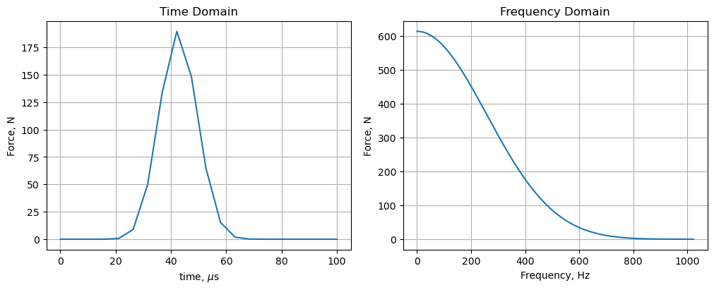
The load represents an explosive bolt in the elbow of the solar array deployment structure on the left. Its time history and spectral content are

Rather than repeating the details here I’ll describe problems I encountered trying to solve the 600k DOF model in MATLAB + dask across 2,048 frequencies using 100 remote workers of Coiled’s cloud.

Aside: Coiled

Coiled is a company created by dask’s founders. It offers dask as a cloud service. Using this service is much easier path than creating a roll-your-own cluster as I did with my 18 anemic DigitalOcean virtual machines. In addition to providing computationally powerful computers, Coiled gives users 10,000 hours of free CPU each month.

I ran this example on Coiled’s cloud.

Sending large amounts of input data to remote workers

If we have a function that takes two input arguments:

result = my_function(argument_1, argument_2)

we can send multiple copies of it to run simultaneously on remote computers with

tasks = []
task = client.submit(my_function, argument_1, argument_2)
tasks.append(task)
task = client.submit(my_function, argument_3, argument_4)
tasks.append(task)
            #   :
            # and so on
            #   :
results = client.gather(tasks)

Dask does many things behind the scenes to make this work. It

1. finds an idle worker to run the function
2. serializes the function arguments then transmits them over the network to the worker
3. deserialized the arguments then instructs the worker to call the function with these arguments
4. captures the return values from the function, serializes them, then transmits them back to the main program where it deserializes them and adds them to the results list

The second step is problematic when the input arguments are massive and don’t change between function calls. In our case the input matrices $K$, $C$, $M$, $P$, and $b$ are invariant and should only be sent over the network once.

Dask has a function for this situation called scatter() which sends the given arguments to all remote computers. It works best when these workers are ready to receive data, so we’ll use another convenience function, wait_for_workers(). The before and after calls are arranged like this:

Python (regular way, without scatter):

tasks = []
client = Client(cluster)
for i in range(n_jobs):
	task = client.submit(solve, K, C, M, b, omega_subset[i])
	tasks.append(task)
results = client.gather(tasks)

Python (with scatter):

tasks = []
client = Client(cluster)
client.wait_for_workers(n_jobs)
KCMb_dist = client.scatter([K, C, M, b], broadcast=True)
for i in range(n_jobs):
	task = client.submit(solve, KCMb_dist, omega_subset[i])
	tasks.append(task)
results = client.gather(tasks)

MATLAB client disconnects

The next problem I encountered was disconnects between the Python worker processes on the remote computers and the dask client in the MATLAB main program. I still don’t know the cause for this although it may be related to the amount of time the computations took on the remote workers.

The solution I came up with was another Python bridge module that contained all dask objects and function calls. Once all dask activity happened in Python, the MATLAB main program ran successfully.

Source code

The MATLAB code to compute the finite element matrices and run the direct frequency domain problem along with the Python bridge module and equation solver are too lengthy to list here. Instead you can find them at my book’s Github repository in these locations:

Performance and cost

The time to solve 2048 frequencies on my 600k DOF model on a single computer in MATLAB is about 8.5 hours. When the MATLAB program distributes the matrices and equation solving step to 100 workers on Coiled’s cloud, the time drops to about 15 minutes, a 33x speed increase.

Concluding remarks

Dask does a lot of work under the hood to make it easy to send work to remote computers. It manages network transmissions of data to and from the workers and balances the load to keep all workers busy. The price for this convenience is a relatively high overhead when tasks are short, that is, less than 10 seconds each. Examples 1 and 2 fall in this relatively wimpy problem class and don’t show dask at its best.

Dask shines on large problems that would otherwise overwhelm a single computer.

Table of Contents | Previous: Accelerate MATLAB with Python and Numba

Accelerate MATLAB with Python and Numba

Part 11 of the Python Is The Ultimate MATLAB Toolbox series.

Lower panel: flow computed with MATLAB 2022b calling the same Navier-Stokes solver translated to Python with Numba. It repeats the simulation more than three times in the amount of time it takes the MATLAB-only solver to do this once.

Introduction

MATLAB’s number crunching power is impressive. If you’re working with a compute-bound application though, you probably want it to run even faster. After you’ve exhausted the obvious speed enhancements like using more efficient algorithms, vectorizing all operations, and running on faster hardware, your last hope may be to to rewrite the slow parts in a compiled language linked to MATLAB through mex. This is no easy task though. Re-implementing a MATLAB function in C++, Fortran, or Java is tedious at best, and completley impractical at worst if the code to be rewritten calls complex MATLAB or Toolbox functions.

Python and Numba are an alternative to mex

In this article I show how Python and Numba can greatly improve MATLAB performance with less effort, and with greater flexibility, than using mex with C++, Fortran, or Java. You’ll need to include Python in your MATLAB workflow, but that’s no more difficult than installing compilers and configuring mex build environments.

Two examples demonstrate the performance boost Python and Numba can bring MATLAB: a simple Mandelbrot set computation, and a much more involved Navier-Stokes solver for incompressible fluid flow. In both cases, the Python augmentation makes the MATLAB application run several times faster.

• Python+Numba as an alternative to mex
• What is Numba?
  • Type casting Python function arguments
  • Options
• Hardware, OS details
• Example 1: Mandelbrot set
• Example 2: incompressible fluid flow
  • Boundary conditions
  • Initial conditions
  • Running the code
  • Visualization

Python+Numba as an alternative to mex

The mex compiler front-end enables the creation of functions written in C, C++, Fortran, Java, and .Net that can be called directly from MATLAB. To use it effectively, you’ll need to be proficient in one of these languages and have a supported compiler. With those in place, the fastest way to begin writing a mex-compiled function is to start with existing working code such as any of the MathWorks' mex examples and modifying it to your needs.

A big challenge to translating MATLAB code is that one line of MATLAB can translate to dozens of lines in a compiled language. Standard MATLAB statements such as

y = max((A\b)*v',[],'all');

become a logistical headache in the compiled languages. Do you have access to an optimized linear algebra library? Do you know how to set up the calling arguments? What if the inputs are complex? What if A is rectangular? It is not straightforward.

Python, on the otherhand, can often match MATLAB expressions one-to-one (although the Python expressions are usually longer). The Python version of the line above is

Python:

y = np.max((np.linalg.solve(A,b).dot(v.T))

where np. is the prefix for the NumPy module.

If you’re familiar with Python and its ecosystem of numeric and scientific modules, you’ll be able to translate a MATLAB function to Python much faster than you can translate MATLAB to any compiled language.

For the most part, numerically intensive codes run at comparable speeds in MATLAB and Python. Simply translating MATLAB to Python will rarely give you a worthwhile performance boost. To see real acceleration you’ll need to additionally use a Python code compiler such as Cython, Pythran, f2py, or Numba.

Numba offers the most bang for the buck—the greatest performance for the least amount of effort—and is the focus of this post.

What is Numba?

From the Numba project’s Overview:

Numba is a compiler for Python array and numerical functions that gives you the power to speed up your applications with high performance functions written directly in Python.

Numba generates optimized machine code from pure Python code using the LLVM compiler infrastructure. With a few simple annotations, array-oriented and math-heavy Python code can be just-in-time optimized to performance similar as C, C++ and Fortran, without having to switch languages or Python interpreters.

Type casting Python function arguments

Three steps are needed to turn a conventional Python function into a much faster Numba-compiled function:

1. Import the jit function and all data types you plan to use from the Numba module. Also import the prange function if you plan to run for loops in parallel.
2. Precede your function definition with @jit()
3. Pass to @jit() type declarations for of each input argument and return value

The steps are illustrated below with a simple function that accepts a 2D array of 32 bit floating point numbers and a 64 bit floating point tolerance, then returns an unsigned 64 bit integer containing the count of terms in the array that are less than the tolerance. We’ll ignore the fact that this is a simple operation in both MATLAB (sum(A < tol)) and Python (np.sum(A < tol)).)

First the plain Python version:

Python:

def n_below(A, tol):
    count = 0
    nR, nC = A.shape
    for r in range(nR):
        for c in range(nC):
            if A[r,c] < tol:
                count += 1
    return count

Now with Numba:

Python:

 1
 2
 3
 4
 5
 6
 7
 8
 9
10

from numba import jit, uint64, float32, float64
@jit(uint64(float32[:,:], float64), nopython=True)
def n_below_numba(A, tol):
    count = 0
    nR, nC = A.shape
    for r in range(nR):
        for c in range(nC):
            if A[r,c] < tol:
                count += 1
    return count

Only the two highlighted lines were added; the body of the function did not change. Let’s see what this buys us:

In : A = np.random.rand(2000,3000).astype(np.float32)
In : tol = 0.5
In : %timeit n_below(A, tol)         # conventional Python
11.3 s ± 72.3 ms per loop (mean ± std. dev. of 7 runs, 1 loop each)

In : %timeit n_below_numba(A, tol)   # Python+Numba
9.92 ms ± 251 µs per loop (mean ± std. dev. of 7 runs, 100 loops each)

Time dropped from 11.3 seconds to 9.92 milliseconds, a factor of more than 1,000. While this probably says more about how slow Python 3.8 is for this problem¹, the Numba version is impressive. It is in fact even a bit faster than the native NumPy version:

In : %timeit np.sum(A < tol)
10.2 ms ± 193 µs per loop (mean ± std. dev. of 7 runs, 100 loops each)

For completeness, MATLAB 2022b does this about as quickly as NumPy:

>> A = single(rand(2000,3000));
>> tol = 0.5;
>> tic; sum(A < tol); toc

Repeating the last line a few times gives a peak (that is, minimum) time of 0.011850 seconds (11.85 ms).

Options

The @jit() decorator has a number of options that affect how Python code is compiled. All four of the options below appear on every @jit() instance in the Navier-Stokes code. Here’s an example:

@jit(float64[:,:](float64[:,:], float64),
     nopython=True, fastmath=True, parallel=True, cache=True)
def DX2(a,dn):
    # finite difference for Laplace of operator in two dimensions
    # (second deriv x + second deriv ystaggered grid)
    return (a[:-2,1:-1] + a[2:,1:-1] + a[1:-1,2:] + a[1:-1,:-2] -
           4*a[1:-1,1:-1])/(dn**2)

nopython=True

Numba compiled functions can work either in object mode, where the code can interact with the Python interpreter, or in nopython mode where the Python interpeter is not used. nopython mode excludes the Python interpreter and results in higher performance.

fastmath=True

This option matches the -Ofast optimization switch used by compilers in the Gnu Compiler Collection. It allows the compiler to resequence floating point computations in a non IEEE 754 compliant manner—enabling significant speed increases at the risk of generating incorrect (!) results.

To use this option with confidence, compare solutions produced with and without it. Obviously if the results differ appreciably you shouldn’t use this option.

parallel=True

This option tells Numba to attempt automatic parallelization of code blocks in jit compiled functions. Parallelization may be possible even if these functions do not explicitly call the prange() to make a for loop run in parallel.

Let’s try this out on the simple n_below() function shown above:

Python:

from numba import jit, prange, uint64, float32, float64
@jit(uint64(float32[:,:], float64), nopython=True, parallel=True)
def n_below_parallel(A, tol):
    count = 0
    nR, nC = A.shape
    for r in prange(nR):    # <-  parallel for loop
        for c in range(nC):
            if A[r,c] < tol:
                count += 1
    return count

By parallelizing the rows of A over cores I get twice the performance on my 4 core laptop:

In : %timeit n_below_parallel(A, tol)
5.96 ms ± 299 µs per loop (mean ± std. dev. of 7 runs, 100 loops each)

Even more impressively, the Navier-Stokes solver runs nearly 2x more quickly with parallel=True on my 4 core laptop even though it has no parallel for loops.

cache=True

A program that includes Numba-enhanced Python functions start more slowly because the jit compiler needs to compile the functions before the program can begin running. The delay is barely noticable with small functions.

That’s not the case for the more complicated jit-compiled functions in the Navier-Stokes solver. These impose a 10 second start-up delay on my laptop. The cache=True option tells Numba to cache the result of its compilations for immediate on subsequent runs. The code is only recompiled if any of the @jit decorated functions change.

Hardware, OS details

The examples were run on a 2015 Dell XPS13 laptop with 4 cores of i5-5200U CPU @ 2.2 GHz and 8 GB memory. The OS is Ubuntu 20.04. MATLAB 2022b was used but the code will run with any MATLAB version from 2020b onward.

Anaconda Python 2020.07 with Python 3.8.8 was used to permit running on older versions of MATLAB, specifically 2020b. (Yes, I’m aware Python 3.11 runs more quickly than 3.8. MATLAB does not yet support that version though.)

Example 1: Mandelbrot set

This example comes from the High Performance Computing chapter of my book. There I implement eight versions of code that compute terms of the Mandelbrot set: MATLAB, Python, Python with multiprocessing, Python with Cython, Python with Pythran, Python with f2py, Python with Numba, and finally MATLAB calling the Python/Numba functions.

The baseline MATLAB version is much faster than the baseline Python implementation. However, employing any of the compiler-augmented tools like Cython, Pythran, f2py, or Numba turns the tables and makes the Python solutions much faster than MATLAB.

baseline MATLAB² :

 1
 2
 3
 4
 5
 6
 7
 8
 9
10
11
12
13
14
15
16
17
18
19
20
21
22
23
24
25
26
27
28
29
30
31
32
33
34
35
36
37

% file: MB_main.m
main()

function [i]=nIter(c, imax)
  z = complex(0,0);
  for i = 0:imax-1
    z = z^2 + c;
    if (real(z)^2 + imag(z)^2) > 4
        break
    end
  end
end

function [img]=MB(Re,Im,imax)
  nR = size(Im,2);
  nC = size(Re,2);
  img = zeros(nR, nC, 'uint8');
% parfor i = 1:nR % gives worse performance
  for i = 1:nR
    for j = 1:nC
      c = complex(Re(j),Im(i));
      img(i,j) = nIter(c,imax);
    end
  end
end

function [] = main()
  imax = 255;
  for N = [500 1000 2000 5000]
    tic
    nR = N; nC = N;
    Re = linspace(-0.7440, -0.7433, nC);
    Im = linspace( 0.1315,  0.1322, nR);
    img = MB(Re, Im, imax);
    fprintf('%5d %.3f\n',N,toc);
  end
end

baseline Python:

 1
 2
 3
 4
 5
 6
 7
 8
 9
10
11
12
13
14
15
16
17
18
19
20
21
22
23
24
25
26
27
28
29
30
31
32
33

#!/usr/bin/env python3
# file: MB.py
import numpy as np
import time
def nIter(c, imax):
  z = complex(0, 0)
  for i in range(imax):
    z = z*z + c
    if z.real*z.real + z.imag*z.imag > 4:
      break
  return np.uint8(i)

def MB(Re, Im, imax):
  nR = len(Im)
  nC = len(Re)
  img = np.zeros((nR, nC), dtype=np.uint8)
  for i in range(nR):
    for j in range(nC):
      c = complex(Re[j], Im[i])
      img[i,j] = nIter(c,imax)
  return img

def main():
  imax = 255
  for N in [500,1000,2000,5000]:
    T_s = time.time()
    nR, nC = N, N
    Re = np.linspace(-0.7440, -0.7433, nC)
    Im = np.linspace( 0.1315,  0.1322, nR)
    img = MB(Re, Im, imax)
    print(N, time.time() - T_s)

if __name__ == '__main__': main()

The Python with Numba version is the same as the baseline Python version with five additional Numba-specific lines. An explanation of each highlighted line appears below the code:

Python with Numba:

 1
 2
 3
 4
 5
 6
 7
 8
 9
10
11
12
13
14
15
16
17
18
19
20
21
22
23
24
25
26
27
28
29
30
31
32
33
34
35
36
37

#!/usr/bin/env python3
# file: MB_numba.py
import numpy as np
import time
from numba import jit, prange, uint8, int64, float64, complex128
@jit(uint8(complex128,int64), nopython=True, fastmath=True)
def nIter(c, imax):
  z = complex(0, 0)
  for i in range(imax):
    z = z*z + c
    if z.real*z.real + z.imag*z.imag > 4:
      break
  return i

@jit(uint8[:,:](float64[:], float64[:],int64), nopython=True,
                fastmath=True, parallel=True)
def MB(Re, Im, imax):
  nR = len(Im)
  nC = len(Re)
  img = np.zeros((nR, nC), dtype=np.uint8)
  for i in prange(nR):
    for j in range(nC):
      c = complex(Re[j], Im[i])
      img[i,j] = nIter(c,imax)
  return img

def main():
  imax = 255
  for N in [500, 1000, 2000, 5000]:
    T_s = time.time()
    nR, nC = N, N
    Re = np.linspace(-0.7440, -0.7433, nC)
    Im = np.linspace( 0.1315,  0.1322, nR)
    img = MB(Re, Im, imax)
    print(N, time.time() - T_s)

if __name__ == '__main__': main()

Line 5 imports the necessary items from the numba module: jit() is a decorator that precedes functions we want Numba to compile. prange() is a parallel version of the Python range() function. It turns regular for loops into parallel for loops where work is automatically distributed over the cores of your computer. The remaining items from uint8 to complex128 define data types that will be employed in function signatures.

Line 6 defines the signature of the nIter() function as taking a complex scalar and 64 bit integer as inputs and returning an unsigned 8 bit integer. (The remaining keyword arguments like nopython= were explained above.)

Lines 15 and 16 define the signature of the MB() function as taking a pair of 1D double precision arrays and a scalar 64 integer and returning a 2D array of unsigned 8 bit integers.

Line 21 implements a parallel for loop; iterations for different values of i are distributed over the cores.

What have we gained with the five extra Numba lines? This table shows how our three codes perform for different image sizes; times are in seconds.

The Python+Numba performance borders on the unbelievable—but don’t take my word for it, run the three implementations yourself!

One “cheat” the Python+Numba solution enjoys is that its parallel for loop takes advantage of the four cores on my laptop. I tried MATLAB’s parfor parallel for loop construct but, inexplicably, it runs slower than a conventional sequential for loop. Evidently multiple cores are only used if you have a license for the Parallel Computing Toolbox (which I don’t).

MATLAB + Python + Numba

If Python can run faster with Numba, MATLAB can too. All we need to do is import the MB_numba module and call its jit-compiled MB() function from MATLAB:

MATLAB:

 1
 2
 3
 4
 5
 6
 7
 8
 9
10
11
12

% file: MB_python_numba.m
np = py.importlib.import_module('numpy');
MB_numba = py.importlib.import_module('MB_numba');
imax = int64(255);
for N = [500 1000 2000 5000]
    tic
    nR = N; nC = N;
    Re = np.array(linspace(-0.7440, -0.7433, nC));
    Im = np.array(linspace( 0.1315,  0.1322, nR));
    img = py2mat(MB_numba.MB(Re, Im, imax));
    fprintf('%5d %.3f\n',N,toc);
end

MB() from MB_numba.py is a Python function so it returns a Python result. To make the benchmark against the baseline MATLAB version fair, the program includes conversion of the NumPy img array to a MATLAB matrix (using py2mat.m) in the elapsed time. The table below repeats the MATLAB baseline times from the previous table. Numeric values in the middle and right column are elapsed time in seconds.

Visualizing the result

Call MATLAB’s imshow() or imagesc() functions on the img matrix if you want to see what the matrix looks like. For example,

MATLAB:

1
2
3
4
5
6
7
8
9

% file: MB_view.m
np = py.importlib.import_module('numpy');
MB_numba = py.importlib.import_module('MB_numba');
imax = int64(255);
nR = 2000; nC = 2000;
Re = np.array(linspace(-0.7440, -0.7433, nC));
Im = np.array(linspace( 0.1315,  0.1322, nR));
img = py2mat(MB_numba.MB(Re, Im, imax));
imagesc(img)

Similarly, in Python:

 1
 2
 3
 4
 5
 6
 7
 8
 9
10
11
12

#!/usr/bin/env python3
# file: MB_view.py
import numpy as np
from MB_numba import MB
import matplotlib.pyplot as plt
imax = 255
nR, nC = 2000, 2000
Re = np.linspace(-0.7440, -0.7433, nC)
Im = np.linspace( 0.1315,  0.1322, nR)
img = MB(Re, Im, imax)
plt.imshow(img)
plt.show()

Example 2: incompressible fluid flow

The Mandelbrot example is useful for demonstrating how to use Numba and for giving insight to the performance boosts it can give. But useful as a computational pattern resembling real work? Not so much.

The second example represents computations as might appear in a realistic scientific application. It demonstrates MATLAB+Python+Numba with a two dimensional Navier-Stokes solver for incompressible fluid flow. I chose an implementation by Jamie Johns which shows MATLAB at its peak performance using fully vectorized code. While this code only computes flow in 2D, the sequence of calculations and memory access patterns are representative of scientific and engineering applications. Jamie Johns' YouTube channel has interesting videos produced with his code.

Boundary conditions

A clever aspect of Jamie Johns' code is that boundary conditions are defined graphically. You create an image, for example a PNG, where colors define properties at each grid point: black = boundary, red= outflow (source), and green = inflow (sink). The image borders, if they aren’t already black, also define boundaries.

This PNG image, which can be found in the original code’s Github repository as scenario_sphere2.png, represents flow moving from left to right around a circle, a canonical fluid dynamics problem I studied as an undergrad:

Of course, if boundary conditions are supplied as images, they can be arbitrarily complex. I recalled an amusing commercial by Maxell, “Blown Away Guy”, from my youth. With a bit of photo editing I converted

to the following boundary conditions image:

The domain dimensions are 15 meters x 3.22 meters and the CFD mesh has 400 x 86 grid points, giving a relatively coarse resolution of 3.7 cm between points. My memory-limited (8 GB) laptop can’t handle a finer mesh.

Initial conditions

• time step: 0.003 seconds
• number of iterations: 12,900
• air density = 1 kg/m$^3$
• dynamic viscosity = 0.001 kg/(m s)
• air speed leaving the speaker: 0.45 m/s

The low air speed is admittedly contrived and certainly lower than the commercial’s video suggests. (my guess is for that is at least 2 m/s). I found the solver fails to converge, then exits with an error, if the flow speed is too high. Same thing for number of iterations—too many and the solver diverges. Trial and error brought me to 0.45 m/s and 12,900 iterations as values that produce the longest animation.

I don’t understand the reason of the failure (mesh too coarse?) and haven’t been motivated to figure out what’s going on. This is, after all, an exercise in performance tweaking rather than studying turbulence or computing coefficients of drag.

Running the code

My modifications to Jamie Johns' MATLAB code and the translation to Python + Numba can be found at https://github.com/AlDanial/matlab_with_python/, under performance/fluid_flow (MIT license). The code there can be run three ways: entirely in MATLAB, entirely in Python, or with MATLAB calling Python.

One thing to note is that the computational codes are purely batch programs that write .mat and .npy data files. No graphics appear. The flow can be visualized with a separate post-processing step after the flow speeds are saved as files.

MATLAB (2020b through 2022b)

Start MATLAB and enter the name of the main program, Main, at the prompt. I had to start MATLAB with -nojvm to suppress the GUI (and close all other applications, especially web browsers) to give the program enough memory.

>> Main

Python + Numba

On Linux and macOS, just type ./py_Main.py in a console.

On Windows, open a Python-configured terminal (such as the Anaconda console) and enter python py_Main.py.

MATLAB + Python + Numba

Edit Main.m and change the value of Run_Python_Solver to true. Save it, then run Main and the MATLAB prompt.

Operation

Regardless of how you run the code (MATLAB / Python / MATLAB + Python), the steps of operation are the same: the application creates a subdirectory called NS_velocity then populates it with .npy files (Python and MATLAB+Python) or .mat files (pure MATLAB). These files contain the x and y components of the flow speed at each grid point for a batch of iterations.

The first time the Python or MATLAB+Python program starts, expect to see delay of about 30 seconds while Numba compiles the @jit decorated functions in navier_stokes_functions.py. This is a one-time cost though; subsequent runs will start much more quickly.

Performance

MATLAB runs more than three times faster using the Python+Numba Navier-Stokes solver. More surprisingly, Python without Numba also runs faster than MATLAB. I updated the performance table on 2022-10-30 following a LinkedIn post by Artem Lenksy asking how the recently released 3.11 version fares on this problem. Numba is not yet available for 3.11 so I reran without @jit decorators—and threw in a 3.8.8 run without Numba as well:

Two surprises here: plain Python + NumPy is faster than MATLAB, and Python 3.11.0 is no faster than 3.8.8 for this compute-bound problem.

Visualization

The program animate_navier_stokes.py generates an animation of flow computed earlier with py_Main.py or Main.m. The most direct way to use it is by giving it the directory (NS_velocity by default) containing flow velocity files and whether you want to see *.mat files generated by MATLAB (use --matlab) or *.npy files generated by either Python or the MATLAB+Python combination (use --python). (Note: the program loads many Python modules and takes a long time to start the first time.)

./animate_navier_stokes.py --python NS_velocity

With this command the program first loads all *.npy files in the NS_velocity directory, then writes a large merged file (merged_frames.npy, 1.7 GB) containing the entire solution in one file. You can later load the merged file much more quickly than reading the individual *.npy files.

The first thing you’ll notice is the animation proceeds slowly. To speed things up, skip a few frames. The next command reads from the merged frame file and only shows every 50th frame:

./animate_navier_stokes.py --npy merged_frames.npy --incr 50

Use the --png-dir switch to write individual frames to PNG files in the given directory. For example

./animate_navier_stokes.py --npy merged_frames.npy --png-dir PNG --incr 400

will create the directory PNG then populate it with 33 files with names like PNG/frame_08000.png. I created the video at the top of this post by saving individual frames, overlaying the Maxell image on each, then generating an MP4 file with ffmpeg.

Table of Contents | Previous: Symbolic math | Next : Distribute MATLAB Computations To Python Running on a Cluster